
Model Distillation: Simplifying AI Models Without Losing Accuracy
- Mr. Data Bugger
- Feb 22
- 4 min read
Model compression refers to techniques that reduce the size and computational cost of deep learning models while maintaining accuracy. This is crucial for deploying AI on edge devices, mobile applications, and low-power environments.
1. Knowledge Distillation
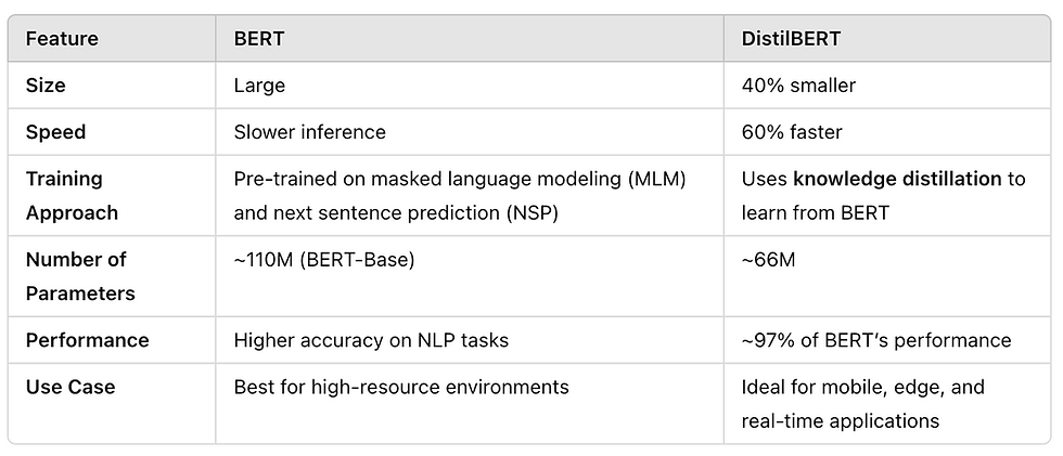
A small student model is trained to imitate a larger teacher model by learning from its soft labels. This reduces model complexity while preserving performance. Example: BERT → DistilBERT.
2. Quantization
Weights and activations are converted from 32-bit floating point (FP32) to lower precision formats like INT8 or FP16, reducing model size and speeding up inference. Used in mobile AI applications.
3. Pruning
Unimportant weights or entire neurons are removed from the network, reducing redundancy. It can be structured (entire layers) or unstructured (individual weights). Often combined with quantization.
4. Low-Rank Factorization
Weight matrices are decomposed into smaller matrices using techniques like Singular Value Decomposition (SVD), reducing computation while keeping model performance stable.
5. Weight Sharing
Similar weights are grouped together and stored efficiently, minimizing redundancy without significantly affecting model accuracy.
Choosing the Right Technique
The best approach depends on the use case. Distillation is great for smaller models, quantization is ideal for faster inference, and pruning helps in deploying lightweight models. A combination of these techniques often yields the best results.
How Model distillation Works
Train a large, powerful model (Teacher Model).
Use the teacher model’s soft predictions (probabilities instead of hard labels) as additional training data.
Train a smaller model (Student Model) to mimic the teacher’s behavior using these soft predictions.
Benefits of Model Distillation
✅ Faster inference – Smaller models run more quickly
.✅ Lower resource usage – Ideal for edge devices and mobile applications
.✅ Improved generalization – Helps reduce overfitting in smaller models.
Example in NLP
Large language models like GPT-4 can be distilled into smaller models like DistilBERT, which retains most of the performance but is much faster.
Types of Distillation based on availability of ground truth
1. Supervised Distillation (with Ground Truth)
The student model learns from both the teacher model’s soft labels and the true labels from the dataset.
This is useful when labeled data is available and helps balance between generalization and accuracy.
Example: Distilling a BERT model into a DistilBERT model while training on a labeled NLP dataset.
2. Self-Distillation / Unsupervised Distillation (No Ground Truth)
The student only learns from the teacher’s soft outputs, without any ground-truth labels.
This is useful when labeled data is scarce or unavailable.
The assumption is that the teacher’s predictions carry useful knowledge even without explicit labels.
Example: Using a large LLaMA model to train a smaller one for chat-based tasks without labeled responses.
Knowledge Distillation in PyTorch
we will guide you through the implementation of knowledge distillation using PyTorch, with a focus on key PyTorch concepts like no_grad(), model.eval(), and train().
🔑 Key Idea
Instead of training the student model on hard labels (ground truth), we also train it using the soft labels provided by the teacher model. This helps the student learn better generalization.
Step 1: Import Required Libraries
import torch
import torch.nn as nn
import torch.optim as optim
import torch.nn.functional as F
from torchvision import datasets, transforms
🔍 Explanation
torch – Core PyTorch library.
torch.nn – Helps in defining models and layers.
torch.optim – Provides optimization algorithms.
torch.nn.functional (F) – Provides activation functions and loss functions.
torchvision.datasets & transforms – Handles dataset loading and preprocessing.
Step 2: Load & Preprocess the Dataset
transform = transforms.Compose([
    transforms.ToTensor(),
    transforms.Normalize((0.5,), (0.5,))
])

train_dataset = datasets.MNIST(root='./data', train=True, transform=transform, download=True)
test_dataset = datasets.MNIST(root='./data', train=False, transform=transform, download=True)

train_loader = torch.utils.data.DataLoader(train_dataset, batch_size=64, shuffle=True)
test_loader = torch.utils.data.DataLoader(test_dataset, batch_size=64, shuffle=False)
🔍 Explanation
transforms.ToTensor() – Converts images to tensors.
transforms.Normalize() – Normalizes pixel values.
DataLoader() – Efficiently loads batches of data for training/testing.
Step 3: Define Teacher & Student Models
Teacher Model (Larger)
class TeacherModel(nn.Module):
    def __init__(self):
        super(TeacherModel, self).__init__()
        self.fc1 = nn.Linear(28*28, 512)
        self.fc2 = nn.Linear(512, 256)
        self.fc3 = nn.Linear(256, 10)

    def forward(self, x):
        x = x.view(-1, 28*28)  # Flatten image
        x = F.relu(self.fc1(x))
        x = F.relu(self.fc2(x))
        x = self.fc3(x)
        return x
Student Model (Smaller)
class StudentModel(nn.Module):
    def __init__(self):
        super(StudentModel, self).__init__()
        self.fc1 = nn.Linear(28*28, 256)
        self.fc2 = nn.Linear(256, 128)
        self.fc3 = nn.Linear(128, 10)

    def forward(self, x):
        x = x.view(-1, 28*28)  # Flatten image
        x = F.relu(self.fc1(x))
        x = F.relu(self.fc2(x))
        x = self.fc3(x)
        return x
🔍 Explanation
Fully connected layers (nn.Linear()) – Define layers of the neural network.
F.relu() – ReLU activation function.
x.view(-1, 28*28) – Flattens images from 28×28 to 784 pixels.
Step 4: Define Loss & Optimizer
teacher = TeacherModel()
student = StudentModel()

criterion = nn.CrossEntropyLoss()
optimizer = optim.Adam(student.parameters(), lr=0.001)
🔍 Explanation
CrossEntropyLoss() – Standard classification loss function.
Adam() – Adaptive learning rate optimizer.
Step 5: Train Teacher Model
def train_teacher(model, train_loader, optimizer, criterion, epochs=5):
    model.train()
    for epoch in range(epochs):
        for images, labels in train_loader:
            optimizer.zero_grad()
            outputs = model(images)
            loss = criterion(outputs, labels)
            loss.backward()
            optimizer.step()
🔍 Key PyTorch Concepts
model.train() – Enables training mode (activates dropout/batch norm).
optimizer.zero_grad() – Clears old gradients.
loss.backward() – Computes gradients for backpropagation.
optimizer.step() – Updates model weights.
Step 6: Train Student Using Knowledge Distillation
def train_student(teacher, student, train_loader, optimizer, criterion, alpha=0.5, T=3):
    teacher.eval()

    for images, labels in train_loader:
        optimizer.zero_grad()

        with torch.no_grad():
            teacher_outputs = teacher(images)

        student_outputs = student(images)

        hard_loss = criterion(student_outputs, labels)
        soft_loss = nn.KLDivLoss()(F.log_softmax(student_outputs / T, dim=1),
                                   F.softmax(teacher_outputs / T, dim=1))

        loss = alpha * hard_loss + (1 - alpha) * soft_loss
        loss.backward()
        optimizer.step()
🔍 Key PyTorch Concepts
teacher.eval() – Sets teacher model to inference mode.
torch.no_grad() – Prevents gradient computation (saves memory & speeds up inference).
Soft Targets (Temperature Scaling):
F.softmax(teacher_outputs / T, dim=1) – Applies softmax with temperature.
F.log_softmax(student_outputs / T, dim=1) – Log softmax before KL divergence loss.
KLDivLoss() – Measures the divergence between student & teacher predictions.
Step 7: Evaluate Student Model
def evaluate(model, test_loader):
    model.eval()
    correct = 0
    total = 0

    with torch.no_grad():
        for images, labels in test_loader:
            outputs = model(images)
            _, predicted = torch.max(outputs, 1)
            total += labels.size(0)
            correct += (predicted == labels).sum().item()

    print(f'Accuracy: {100 * correct / total:.2f}%')
🔍 Key PyTorch Concepts
model.eval() – Ensures proper inference behavior.
torch.no_grad() – Disables gradients for efficiency.
torch.max(outputs, 1) – Finds highest probability class.
Conclusion
By using knowledge distillation, we successfully trained a smaller, efficient student model that mimics a larger teacher model. This approach is widely used in real-world applications like deploying lightweight models on mobile devices.

Comentarios